Every model so far started with a mechanism: births, deaths, cooling, infection. Sometimes we don’t know the mechanism, but we do have measurements. Can data alone give us a model that makes useful predictions? And how can we tell when that model deserves our trust?
NoteReading and code
Read textbook Module 8.3, “Empirical Models.” Download the two data files and save them in the same folder as your R script: pontius.csv and danwood.csv. In Positron, open that folder (File → Open Folder) so read.csv() can find them. Download the complete R script after coding along.
The datasets come from the National Institute of Standards and Technology (NIST) Statistical Reference Datasets, the same ones the textbook uses.
Explaining vs. predicting
A mechanistic model, like constrained growth or SIR, explains a system. Each term stands for something real, so we can ask “what if?” questions about it.
An empirical model is a function chosen only because it follows the trend of the data. The book’s definition (p. 353): an empirical model “is based only on data and is used to predict, not explain, a system.” It can be very useful, but only where we have data. Outside that range, the data have nothing to say.
A straight line: calibrating a load cell
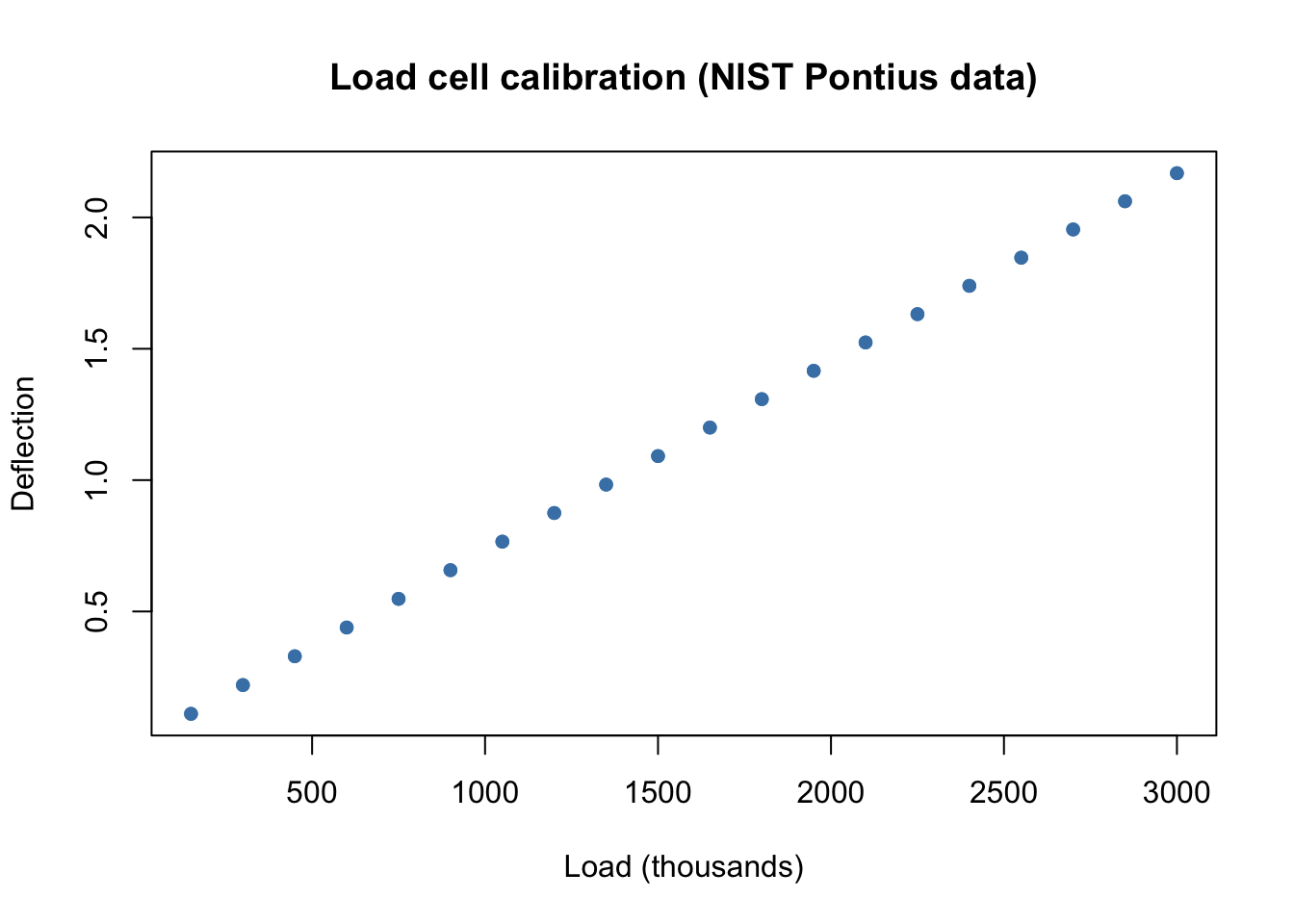
A load cell is a sensor that bends slightly under weight. Engineers at NIST hung known loads on one and recorded the deflection, twice at each of 20 loads. If the relationship is reliable, we can turn any deflection reading into a weight.
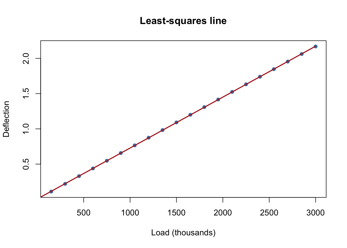
That looks like a line. R’s lm() (“linear model”) finds the least-squares line: the slope and intercept that make the sum of the squared vertical distances from the points to the line as small as possible (pp. 356–357). The formula deflection ~ load_thousands reads “deflection as a function of load.”
line_fit <-lm(deflection ~ load_thousands, data = pontius)coef(line_fit)
The slope says each additional 1,000 units of load adds about 0.00072 to the deflection. To draw the fitted line, ask the model for predictions at many loads with predict():
A load of 1,000 is inside the range we measured (150 to 3,000), so we have good reason to trust that prediction. A load of 10,000 is more than three times the largest load tested. The line happily gives an answer, but would the real sensor stay linear, or bend, or break? The data can’t tell us. Using a model beyond the range of its data is called extrapolation.
Residuals: what the line missed
The line looks perfect. Is it? A residual is the part of each observation the model doesn’t explain:
\[
\text{residual} = \text{observed } y - \text{predicted } y.
\]
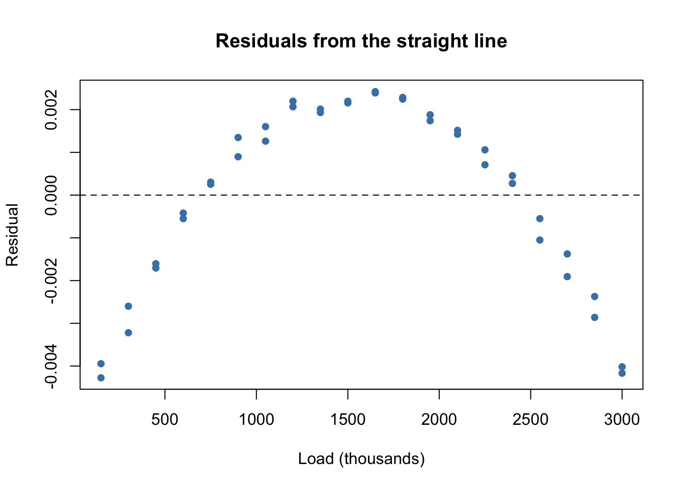
If a model has captured the trend, its residuals should look like random scatter around zero. If they show a pattern, the model is missing something.
plot(pontius$load_thousands, resid(line_fit), pch =16, col ="steelblue",xlab ="Load (thousands)", ylab ="Residual",main ="Residuals from the straight line")abline(h =0, lty =2)
Those residuals form a clear arch: the line is too low in the middle and too high at both ends. The errors are tiny (thousandths), but they aren’t random. The real relationship curves slightly.
lm() can fit any linear combination of terms (p. 354), not just \(b + mx\). Adding an \(x^2\) term gives a quadratic, \(y = b_0 + b_1 x + b_2 x^2\). Inside a formula, I(load_thousands^2) tells R to square the values.
quad_fit <-lm(deflection ~ load_thousands +I(load_thousands^2), data = pontius)coef(quad_fit)
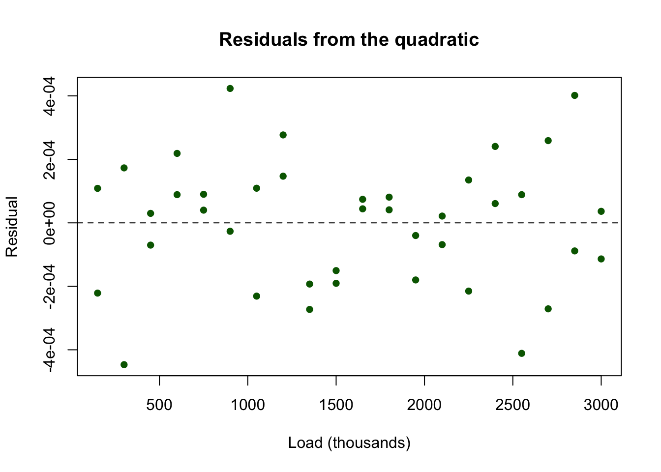
plot(pontius$load_thousands, resid(quad_fit), pch =16, col ="darkgreen",xlab ="Load (thousands)", ylab ="Residual",main ="Residuals from the quadratic")abline(h =0, lty =2)
The arch is gone, and the residuals are about ten times smaller. What’s left looks like measurement noise. The \(x^2\) coefficient is tiny, but it matters at this level of precision. Notice that we found it by looking at the residuals, not at the original plot.
A one-term model: a glowing filament
Our next data relate the temperature of a carbon lamp filament (in thousands of kelvins) to the energy it radiates per square centimeter per second.
danwood <-read.csv("danwood.csv")danwood
  temperature energy
1       1.309  2.138
2       1.471  3.421
3       1.490  3.597
4       1.565  4.340
5       1.611  4.882
6       1.680  5.660
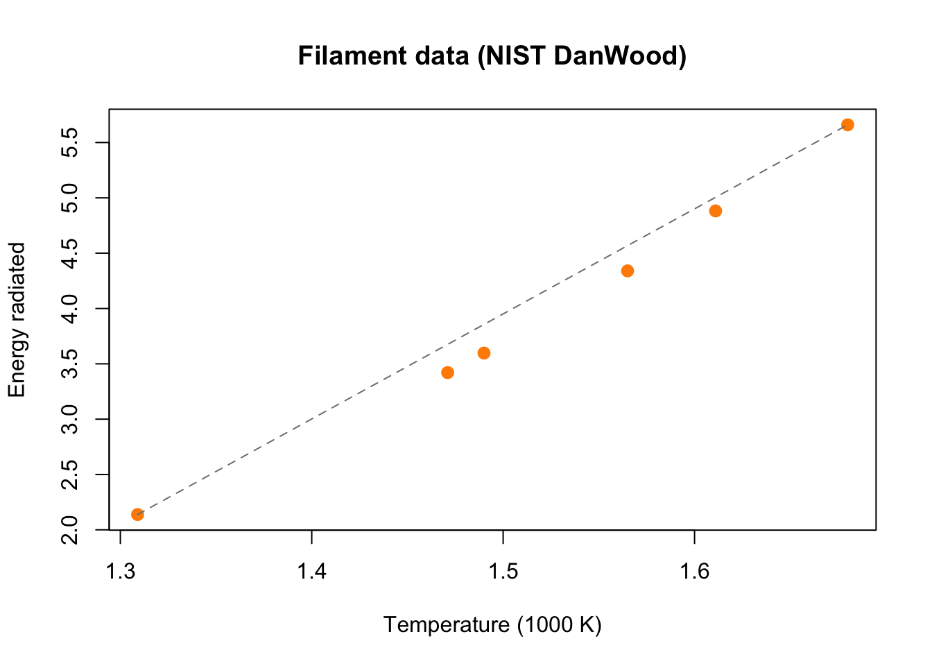
plot(danwood$temperature, danwood$energy, pch =16, cex =1.3,col ="darkorange", xlab ="Temperature (1000 K)",ylab ="Energy radiated", main ="Filament data (NIST DanWood)")lines(range(danwood$temperature), range(danwood$energy), lty =2, col ="gray50")
The dashed line through the first and last points shows that the data curve upward (concave up). The book’s idea (pp. 357–360): find a power \(p\) so that plotting \(y\) against \(x^p\) looks straight. Raising values greater than 1 to a power stretches the larger ones more, which straightens a concave-up pattern. Then fit a line to \((x^p, y)\).
Rather than trying powers by hand, let a loop do it. For each power, fit the line and record the sum of squared residuals (smaller is better):
powers <-seq(1, 5, by =0.5)ssr <-numeric(length(powers))for (k inseq_along(powers)) { z <- danwood$temperature^powers[k] fit <-lm(danwood$energy ~ z) ssr[k] <-sum(resid(fit)^2)}data.frame(power = powers, sum_sq_residuals =round(ssr, 5))
The power 3.5 gives the smallest sum, about 50 times smaller than a straight line (\(p = 1\)). It’s the same power the textbook picks by looking at plots. (Try a finer grid between 3 and 4. Does the best power move much?) Let’s use it:
danwood$temp_power <- danwood$temperature^3.5power_fit <-lm(energy ~ temp_power, data = danwood)coef(power_fit)
(Intercept)  temp_power
 -0.3931313   0.9881859
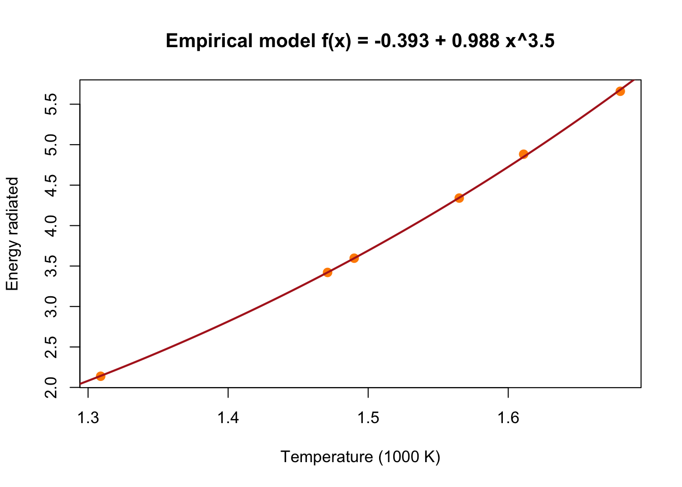
These match the book: \(y = -0.393 + 0.988\,z\) with \(z = x^{3.5}\). Substituting back gives the empirical model
\[
f(x) = -0.393 + 0.988\,x^{3.5}.
\]
Always check the model against the original, untransformed data. Here’s the curve with the measurements:
temp_grid <-seq(1.25, 1.75, by =0.005)plot(danwood$temperature, danwood$energy, pch =16, cex =1.3,col ="darkorange", xlab ="Temperature (1000 K)",ylab ="Energy radiated", main ="Empirical model f(x) = -0.393 + 0.988 x^3.5")lines(temp_grid, -0.393+0.988* temp_grid^3.5, col ="firebrick", lwd =2)
A physics aside: a law from physics (the Stefan–Boltzmann law) says an ideal glowing body radiates energy in proportion to \(T^4\). Our data alone suggested a power near 3.5, close to but not equal to 4. A real filament isn’t an ideal body, and six points can’t pin the exponent down precisely. This is the empirical approach’s strength and weakness at once: it follows these data, without knowing why.
Next time: a perfect fit that’s wrong
So far, adding a term (the \(x^2\) in the load-cell model) made the fit better. Can we keep adding terms? On Wednesday we’ll fit a polynomial that passes through every data point exactly, see why its predictions are absurd, and look for a better way to choose a model in Empirical Models in Practice.
ImportantWhen does an empirical model deserve trust?
Plot the model on the original data, not just the transformed data.
Look at the residuals. A pattern means the model is missing something; random scatter is what we want.
Prefer the simplest model that leaves patternless residuals.
Don’t extrapolate. Outside the range of the data, an empirical model is a guess.
Use what you know. When theory suggests a shape, such as a power law, start there.